Cell Dynamics using CellVista SLIM — Label-Free 3D Cell Structure Tomography

Applications in basic biological sciences, such as cell viability and function, and clinical studies, such as drug testing, require an understanding of the activity of and interactions between the many molecules that make up the complex world the cell. CellVista SLIM provides an ideal means to study the intra- and inter-cellular dynamics by tracking the movement of small organelles or analyzing a region of interest as a whole.
CellVista SLIM’s sub-nanometer sensitivity and diffraction limited resolution enables the quantitative data yield of actual mass transport information, in terms of diffusion coefficients and velocity distributions.
We can produce live demonstrations for this topic, either with in-house samples or delivered samples.
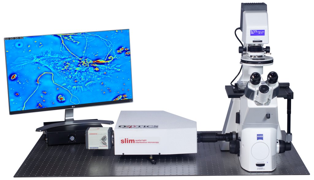
Phi Optics CellVista System seamlessly upgrades the camera port of your microscope for studying Cell Dynamics.
Free Pre-Recorded Webinar
Register to access this free online video webinar which covers this topic in-depth.
for Cell Dynamics
CellVista SLIM is a non-invasive phase imaging technology that quantifies the physical properties of live cells and tissues providing meaningful information regarding cell dynamics. The output is a live quantitative image (SLIM map) of the specimen. The intensity of every pixel in the frame is a measure of a phase shift map (in radians) or the optical path length difference (in nanometers) through the sample, which is measured with sensitivity better than 0.5 nanometers. The phase shift map is converted on-the-fly to other SLIM maps, with their respective pixel intensity: thickness (in microns), dry mass area density (pictograms per square micron) and refractive index. Moreover, the phase shift map can be used for reconstructing the scattering measurement. More detailed description of CellVista SLIM can be found in the reference pages in the How It Works page of this website.
Organelle tracking: CellVista SLIM images reveal the locations of small organelles within the cell. These dense deposits of protein, high in dry mass, can easily be detected, and tracked over a time-lapse measurement. Phi Optics provides a set of plugins based on the NIH ImageJ and Particle Tracker plugin.
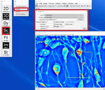
Figure 2. Particle tracking plugin configuration
Particle tracking can be setup and performed using the Particle Tracker plugin. The steps to use the plugin are:
- Load a CellVista SLIM time sequence for tracking the particles (organelles). Particle contrast can also be enhanced by applying Laplacian to the image.
- Run the Particle Tracker plugin in the Dynamics menu.
- Adjust the parameters (Radius, Cutoff, Per/Abs, Link Range, Displacement) and use “Preview Detected” to confirm the detection (Figure 2).
- Plugin will show a result window.
Analysis. Once the plugin finishes particle detection, it shows a result window with a variety of options to display the result.The trajectories of the detected particles can be visualized by “Visualize All Trajectories” in the result window. The trajectories can be saved to a table, which contains the coordinate of each detected particle for each frame, by “All Trajectories to Table” in the result window. Using the coordinates, the Mean Square Displacement (MSD) can be plotted, and MSD vs. time plot yields diffusion coefficient.
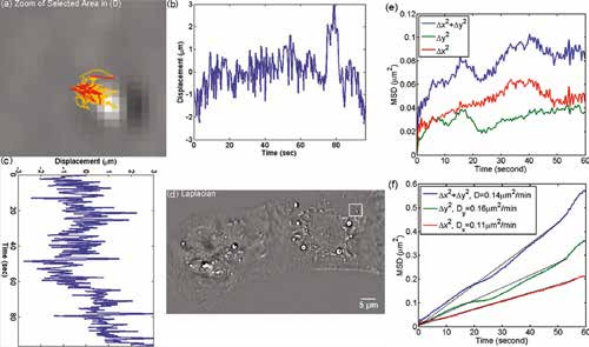
Organelle movement within a beating heart cell. CellVista SLIM was used to track the organelle movement within a beating heart cell. The tracking of organelle allowed for the measurement of the diffusion coefficient. The small diffusion coefficient indicates that the movement of the organelles are restricted by the cell. MSD measurement for particles within the cardiac myocytes in Figure on left: (a) Zoom into the selected area shown in (d); (b) Displacement in Y direction; (c) Displacement in X direction. (d) Laplacian of the phase map; (e) MSD for the particle shown in (a). (f) MSD ensemble-averaged over 15 particles in (d).
Intercellular transport between neurons. Intercellular transport has also been studied using SLIM, by analyzing the transport between neurons [2]. The diffusion coefficient in the horizontal and vertical directions are calculated. Because the neurites are mostly extending horizontally within the field of view, the spatial confinement along the vertical direction resulted in a very small diffusion coefficient along the vertical direction.
A. Obtaining DPS data:
- Load a CellVista SLIM time sequence for DPS analysis
- Run the DPS plugin in the Dynamics menu
- Adjust the parameters (time step and pixel size), select a square ROI to be analyzed and run the plugin
- The result will show a DPS map and a DPS plot
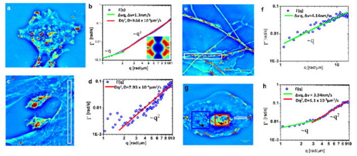
Dispersion-relation Phase Spectroscopy (DPS). CellVista SLIM provides a way to study cellular dynamics even when the dynamic structures are continuous and cannot be tracked as particles. DPS is a method for analyzing SLIM time lapse images. DPS provides a relation between the spatial and temporal fluctuations on the sample, and yields information about the diffusion coefficient, velocity distributions, as well as the mode of transport: random or deterministic.
B. Dispersion-relation phase spectroscopy of inter- and intra-cellular transport
DPS is applied to a variety of cells, including glia, microglia and neurons, to infer the intercellular and intracellular transport of these cells.
The output provides information regarding the diffusion coefficient, advection velocity and the mode of transport.
For high image resolution solutions of thick specimens, please see our CellVista GLIM™ systems. For customization don’t hesitate to CONTACT US!
References:
[1] G. Popescu (2011) Quantitative phase imaging of cells and tissues (McGrow-Hill, New York).
[2] Z. Wang, L. Millet, V. Chan, H. Ding, M. U. Gillette, R. Bashir, and G.Popescu, Label-free intracellular trans- port measured by spatial light interference microscopy, J. Biomed. Opt., 16(2), 026019 (2011).
[3] I. F. Sbalzarini and P. Koumoutsakos. Feature point tracking and trajectory analysis for video imaging in cell biology. J. Struct. Biol., 151(2): 182–195, 2005.
[4] R.Wang, Z. Wang, L. Millet, M. U. Gillette, A.J. Levine, and G.Popescu, Dispersion-relation phase spectros- copy of intracellular transport, Opt. Exp. 19(21), 20571 (2011).