3D Cell Tomography with CellVista SLIM — Label-Free 3D Cell Structure Tomography

CellVista SLIM™ is a non-invasive phase imaging technology that quantifies the 3D cell structure of live cell cultures with single cell resolution. The output is a live quantitative image of the specimen on the microscope stage. The intensity of every pixel in the frame is a measure of the optical path length difference (in radians) through the sample (Phase shift map is measured with better than 0.5 nanometers sensitivity). When used with a high NA objective, the white-light illumination of CellVista SLIM provides an exceptional optical sectioning effect (Figure 1), which allows for imaging a virtual slice of thickness near 1 µm within the cell [2, 3].
In other words, the specimen is virtually sliced into thin pieces and each slice is imaged sequentially as the imaging system scans its focus through the object. The necessary settings in order to perform a z-stack measurement is integrated in Phi Optics Cell Vista software, which controls both the acquisition and the microscope focus scanning.

The result of 3D imaging using SLIM is a stack of images scanned through the focus (z-stack). In order to properly analyze the 3D data, the z-stack needs to be adjusted to take into account the spatial scale represented in the stack, i.e. setting the voxel size for the stack. This can be done by adjusting the properties of the stack in ImageJ. The Properties menu can be found under Image menu of the main ImageJ window, and allows the user to set the width, height and depth. Width and height are the spatial scale on the sample plane that a pixel represents in the SLIM map. Depth is simply the z-step size determined by the experiment.

3D Project generates a 3D rendering from in the form of varying perspectives along the vertical axis. In other words, 3D Project generates 360° rotation of the reconstructed object. The result is a stack of images, each showing a projection of the object at the angle corresponding to the image (Figure 2, above).

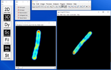
Unlike in the 3D Project, the 3D Viewer user can rotate the volume freely without constraints of 1 axis and zoom in and out. The threshold for transparency can also be applied under the “Edit” menu of the result window. Moreover, the plugin allows the user to input multiple channels for reconstruction, allowing an overlay between multiple imaging modalities.

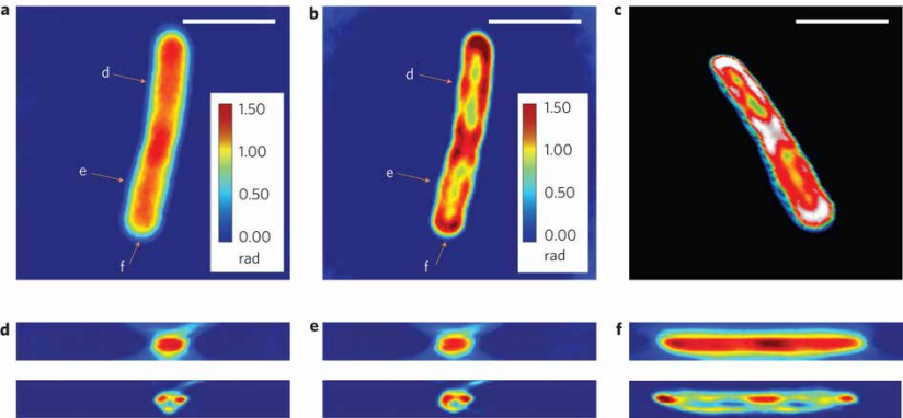
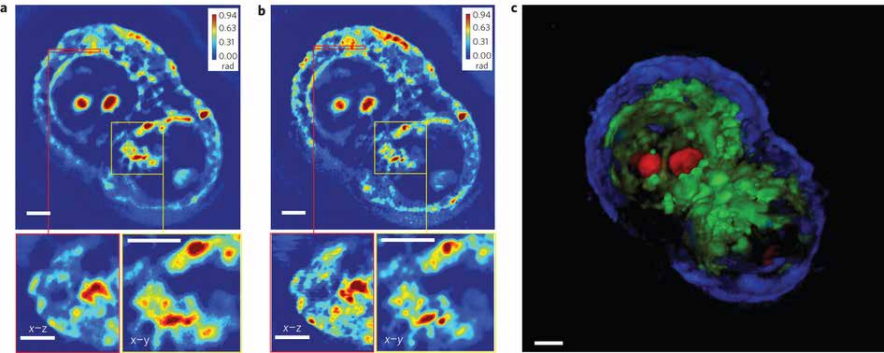
Orthogonal View shows 3 cross-sections along 3 representative planes, x-y, y-z, and x-z, taken at a specified location. The plugin opens 2 windows around the original stack to represent the two orthogonal views of the stack. The cross-section location is indicated by yellow lines, and can be selected by simply clicking on the image or by scanning the z-stack.

Volume Viewer provides 3D rendering of a stack and also shows the cross-sections along x-y, y-z, x-z planes. There are several modes of operation: Slice, Slice & Borders, Max Projection, Projection and Volume. Slice and Slice & Borders show one slice orthogonal to the line of sight of the user. Max Projection and Projection shows one perspective which represents the maximum or the average values along the line of sight. 

Volume constructs a 3D object from the stack, similarly to the 3D viewer (Figure 5). The user can adjust the alpha, or the transparency, of the whole stack easily by drawing an own curve on the histogram located on the right side of the result window.

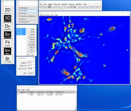
Cell Volume Plugin: Provides an easy method for determining the volume of a cell when used with a low NA objective. The volume at each pixel can be calculated, and by integrating these volumes over the area covered by the cell, the cell volume can be determined. An ImageJ plugin calculates the cell volume from the phase map.

Using Deconvolution to Improve 3D Cell Tomography

In order to improve the image quality and resolution, the 3D stack can be deconvolved using the system point spread function (PSF), which can be calculated or measured using a small bead [2,3]. The result yields suppressed out-of-focus lights and better resolution, and thus, allows the user to see smaller details of the specimen (Figure 7 and Figure 8). Deconvolution can be performed using the DeconvoluionJ plugin under 3D Analysis menu. 

Two tomograms obtained by CellVista SLIM with deconvolution are introduced below.

Figure 7 (Left). White-light Diffraction Tomography (WDT) of E.) coli cells is shown. (a) The center frame of a z-stack measurement using a ×63/1.4 NA oil immersion objective.
(b) Deconvolution result of the same z-slice as in a, clearly showing a resolved helical structure.
(c) Centre cut of the three-dimensional rendering of the deconvolved z-stack, which shows both the overall cylindrical morphology and a helical subcellular structure.
(d–f) Cross-sections of the measured z-stack (top row) and the deconvolved z-stack (bottom row). Each figure label corresponds to the markers shown in a,b and is in the same scale as a,b. Scale bars, 2mm. A z-stack of 17 images, each with 128×128 pixels is used for the reconstruction, which requires about 3 min for sparse deconvolution.

Figure 8 (right). (a) A measured z-slice (top), a cross-section at the area indicated by the red box (bottom left) and a zoomed-in image of the area indicated by the yellow box (bottom right), measured using a ×63/1.4 NA oil immersion objective. (b) A deconvolved z-slice corresponding to the measurement shown in a (top), a cross-section at the area indicated by the red box (bottom left) and a zoomed-in image of the area indicated by the yellow box (bottom right). By comparing a and b, the resolution increase can be clearly seen. (c) False-colour three-dimensional rendering of the deconvolution result (Supplementary Movie 3). We used z-stacks of 140 images, each with a dimension of 640 × 640. Owing to the large image dimension, the image is split into 25 sub-images for faster deconvolution. Overall, the deconvolution process took approximately an hour. Scale bars in all panels, 5 µm.

For high image resolution solutions of thick specimens, please see our CellVista GLIM™ systems. For customization don’t hesitate to CONTACT US!